Equation 1
Note:
2. Augmenting Reality with Minimal Calibration
This section describes a new approach to augmenting reality that moves away from relating all reference frames to a common Euclidean 3D reference frame. Instead the camera, real world and virtual objects are specified in an affine representation. Four non-coplanar points in the scene define this affine frame. The technique utilizes the following property of affine point representations (Koenderink and van Doorn 1991; Ullman and Basri 1991): Given a set of four or more non-coplanar 3D points represented in an affine reference frame, the projection of any point in the set can be computed as a linear combination of four points in the set. The affine representation allows the calculation of a point's projection without the requirement of having any information about the camera position or its calibration parameters. It does, however, represent only those properties of an object that are preserved under an affine transformation. Under an affine transformation lines, intersections of lines and planes and parallelism are preserved.
For use in an augmented reality application Uenohara and Kanade (Uenohara and Kanade 1995) have suggested the use of geometric invariants. Their description used planar invariants and 2D overlays for the augmented image. This work extends that to include 3D rendering and placement of arbitrary virtual objects. The problem of correctly merging a virtual image with an image of a real scene is reduced to:
Accurate determination of where a virtual point and a real point in 3D space will project on their respective image planes is essential so that the two image planes can be correctly overlaid (Foley, van Dam et al. 1990; Tuceryan, Greer et al. 1995). This requires a knowledge of the relationships between the reference frames shown in Figure 4. More specifically, if [X Y Z 1]T are the homogeneous coordinates for a virtual point and [u v 1]T are its projection in the graphics image plane, the projection process can be expressed as:
Equation 1
where O3x4 is the homogeneous transformation from virtual object coordinates to world coordinates, C4x4 is the transformation from world coordinates to graphics camera coordinates and P4x4 describes the projection operation of the synthetic graphics camera onto the graphics image plane. A similar expression exists for the projection of a real point to the image plane of the camera. Equation (1) assumes that each of the reference frames is independently defined and not related to each other. In the U of R augmented reality system, all frames are defined in a common affine coordinate frame. That frame is defined by four non-coplanar points that are in the camera view and can be visually tracked through all video frames.
With this representation the projection process can be expressed as a single homogeneous transformation for both virtual points and real points in space:
Equation 2
where [x y z 1]Tare the affine coordinates of the point transformed from [X Y Z 1]T and P3x4 defines the overall projection of a 3D affine point onto the image plane.
This has now shifted the problem of determining the correct projection of the virtual objects from one that requires multiple reference frames to be precisely related, to one of transforming all reference frames to the common affine reference frame and then calculating the single affine projection matrix, P, for each new view of the scene. The techniques for accomplishing this will be discussed in the following sections.
All points in the system are represented in an affine reference frame. This reference frame is defined by 4 non-coplanar points, p0 ... p3. The origin is taken as p0 and the affine basis points are defined by p1, p2 and p3. The origin, p0 is assigned homogeneous affine [0 0 0 1]T coordinates and basis points, p1, p2, p3 are assigned affine coordinates of [1 0 0 1]T, [0 1 0 1]T, [0 0 1 1]T respectively. The associated affine basis vectors are p1 = [1 0 0 0]T, p2 = [0 1 0 0]T, and p3 = [0 0 1 0]T. Any other point, px, is represented as px = xp1 + yp2 + zp3 + p0 where [x y z 1]T are the homogeneous affine coordinates for the point. This is a linear combination of the affine basis vectors.
Affine reprojection (Koenderink and van Doorn 1991; Mundy and Zisserman 1992) is used by the U of R system to create the projection of any other point defined in the affine coordinate frame. The general process of reprojection is:
Given the projection of a collection of 3D points at two positions of the camera, compute the projection of these points at a new third camera position.
A weak perspective projection model for the camera is used to approximate the perspective projection process. The use of an affine representation for the points allows the calculation of the reprojection of any affine point without knowing the position or internal calibration parameters for the camera. Only the projections of the four points defining the affine frame are needed to determine P in Equation 2. The reprojection property, illustrated in Figure 8, is expressed as:
If in an image, Im, the projection, [upi vpi 1]T of the four points, pi i = 0 ... 3, which define the affine basis is known then the projection, [up vp 1]T of any point, p, with homogenous affine coordinates [x y z 1]T can be calculated as
Equation 3
Figure 8 - Affine Point Reprojection
Equation 3 provides an explicit definition for the projection matrix P seen in Equation 2. It provides the method to easily compute the projection of a 3D point in any new image being viewed by the camera as a linear combination of the projections of the affine basis points. To do this we require the location of the image projection of the four points defining the affine frame and the homogeneous affine coordinates for the 3D point. Visual tracking routines initialized on the feature points that define the affine frame provide the location values. The next section describes the technique for initially determining the affine coordinates for any 3D point in the current affine frame.
The affine reconstruction property (Koenderink and van Doorn 1991; Mundy and Zisserman 1992) can be stated as:
The affine coordinates of any point can be computed from Equation 3 if its projection in at least two views is known and the projections of the affine basis points are also known in those views.
This results in an over-determined system of equations based on Equation 3. Given two views, I1, I2, of a scene in which the projections of the affine basis points, p0, ..., p3, are known then the affine coordinates [x y z 1]T for any point p can be found from the solution of the following equation:
Equation 4
where [up vp 1]T and [upi vpi 1]T are the projections of point p and affine basis point pj, respectively, in image Ii.
Affine DepthOne of the performance goals for an augmented reality system is the ability to operate in real-time. Computing resources are needed for tracking basis points as required by the affine formulations presented above and for generating the virtual images that augment the real image. Generating the virtual image relies on well developed rendering algorithms (Foley, van Dam et al. 1990). Computer graphic systems provide hardware support for rendering operations that enable real-time rendering of complex graphic scenes. Obviously, an augmented reality system should use hardware support when it is available. Hidden surface removal via z-buffering is a primary operation supported by hardware. Z-buffering requires an ordering in depth of all points that project to the same pixel in the graphics image. This is usually done by giving each point a value for its depth along the optical axis of the synthetic graphics camera. The affine point representation in which all points are defined in this system preserves depth order of the points. In rendering the virtual objects with an orthographic graphics camera, the magnitude of this z-value is irrelevant only the order of points must be maintained.
To obtain a depth ordering, first determine the optical axis of the camera as the 3D line whose points all project to the same point in the image. The optical axis is specified as the homogeneous vector [zT 0]T where z is given as the cross product
Equation 5
These two vectors are the first three elements of the first and second rows of the projection matrix P. A translation of any point p along this direction is represented as p' = p + a[zT 0]T. The projection in the image plane of each of these points is the same as the projection of p.
The depth value used for z-buffering is assigned to every point p as the dot product p[zT 0]T. This allows the complete projection of an affine point to be expressed as
Equaiton 6
This has the same 4x4 form as the viewing matrix that is commonly used in computer graphics systems to perform transformations of graphic objects. The difference between the affine projection matrix and the graphics system viewing matrix is in the upper left 3x3 submatrix. In Equation 6 that submatrix is a general invertible transformation whereas when working with a Euclidean frame of reference it is a rotation matrix. The structural similarity, however, allows standard graphics hardware to be used for real-time rendering of objects defined in the affine frame of reference developed here. The power of a graphics processor such as the Silicon Graphics Reality Engine can be directly used to perform object rendering with z-buffering for hidden surface removal.
A prototype augmented reality system (Kutulakos and Vallino 1996; Kutulakos and Vallino 1996; Kutulakos and Vallino 1996) has been constructed using the techniques described in the previous section. It demonstrates that a live video scene can be augmented with computer graphic images in real time. Regions in the image are tracked to determine the projections of the affine basis points and, in turn, calculate the affine projection matrix for each new view. The current system runs as multiple processes on two machines communicating over an Ethernet connection. While there are limitations in the current system, as described in Section 3.1, the system does demonstrate the basic feasibility of this approach to augmented reality. The next sections will describe the system components and operation along with some performance measurements that have been made.
The design of this prototype augmented reality system very closely follows the architecture for a typical augmented reality system given in Figure 4. A block diagram of the components in this system is shown in Figure 9.
Figure 9 - University of Rochester Prototype Augmented Reality System Block Diagram
Standard consumer grade camcorders manufactured by Sony Corporation are used for
viewing the real scene. The output of these cameras goes to two locations. The first
location is a pair of MaxVideo 10 frame grabbers, manufactured by Datacube Inc., used for
digitizing the video frames. None of the advanced image processing hardware available with
this series of video boards is used. They are only used in the capacity of video
digitizers. Two cameras are used during the initialization of the system to provide
simultaneously the two views of the scene needed for performing affine reconstruction.
While the system is running (see Section 2.6.2)
only one camera is needed to calculate the affine projection matrix for each new view. The
output from this camera also goes to the video keyer responsible for mixing the real and
virtual video images.
Two region trackers running as separate processes on the SPARCserver use the digitized images to determine the locations of feature points in the image and calculate the affine projection matrix for subsequent views from either camera. These region trackers use robust statistical estimation and Kalman filtering to track the edges of two four-sided regions at video frame rate, i.e. 30 Hz. Communication with each tracker processes is via a socket interface. After initialization, the trackers track the edges of the regions specified and determine the feature points by calculating their position from the boundaries of those regions. The location of the affine basis points is determined and used to create the affine projection matrix for each new view. The updated projection matrix is made available to the rest of the system through the sockets interface to the trackers.
A graphics server process runs on the Silicon Graphics machine using the Reality Engine for rendering of the scene. This program is a mixed OpenGL and Open Inventor application (Silicon Graphics Inc. 1992; Silicon Graphics Inc. 1994). An Open Inventor scene file defines the basic structure for the graphics operations. All virtual objects to be rendered are also described using the Open Inventor file format. Communications to the graphics server is via a sockets interface. The graphics server renders the virtual objects into a window that is 640 x 480 and is available externally as a VGA signal. Merging of the real and virtual scenes is done in hardware by luminance keying. The luminance keyer gets two inputs. The virtual image is its key input and the image of the real scene is the reference input. The reference input serves two purposes. First, the reference input provides the background signal for the luminance key. The graphics system renders the virtual objects against a background whose intensity is below the luminance key level. The video image of the real scene will appear in the augmented image in all of these background areas. Wherever a virtual object has been drawn that object will overlay the real video image in the output. Example augmented reality displays are shown in Section 2.6.2. The reference input also serves as the synch signal for the keyer. The keyer output is the augmented video image and is synchronized to the reference input. This will be useful later for further video processing of that image.
This section will describe the operation of this prototype augmented reality system. The previous section discussed the hardware and software components and how they were connected. Here the process of initialization of the system from the user's perspective is discussed along with some pertinent issues concerning interactions with the graphics system.
The augmented reality system is controlled from a Matlab process that starts up the graphics server process and two trackers. The first step is determining the relationship between pixel locations in the graphics system and the digitizers used by the trackers. This is performed by digitizing the alignment pattern shown in Figure 10 and having the user specify the digitized pixel location in Matlab of the three alignment marks.
Figure 10 - Digitized Alignment Pattern
The graphics server provides the location of the fiducials in its window and the transformation, Tgi, between digitized image frame and graphics frame is obtained by solving
![]()
Equation 7
where g1, g2, g3 are the positions used by the graphics server when rendering the alignment marks and i1, i2, i3 are the corresponding projections in the digitized image.
The trackers each receive video input from a video camcorder viewing the scene. The user initializes each tracker to track two rectangular regions. The tracked regions are outlined on the output image for each tracker. After the second tracker is initialized data is exchanged between the two trackers and the location of the affine basis points and the affine frame of reference is computed. Note that the system can also be initialized with a single camera. In that case, it is necessary to move the camera, or if possible move the tracked regions, to provide the second view that is needed for initialization of the system. The view from an operating tracker is shown in Figure 11. Note that the two regions being tracker are outlined, and the axes for the affine basis that has been chosen is also shown. As the small frame is moved around in front of the cameras the user gains a sense for the orientation of the affine basis.
![]()
Figure 11 - Region Tracker in Operation
Having defined the affine frame, the next step is to place the virtual objects into the image. Remember that the camera, real scene and virtual scene are defined in the same affine reference frame. Models of objects are defined using the Open Inventor (Silicon Graphics Inc. 1994) file format. The models available are defined in a more common Euclidean frame. To use these object models a transformation into the current affine frame will need to be calculated. The user interactively defines to the system where the virtual object should be placed in the scene. The position is defined by specifying the location of the x, y, z axes and the origin of a Euclidean bounding box for the object. This specification is done in both views of the scene. From these four point correspondences in two images, the affine coordinates for the points, ax, ay, az, ao, can be computed using the affine reconstruction property (Section 2.4). Assuming that the Euclidean bounding box is of unit size, the transformation, Tae from the bounding box frame to the current affine frame can be calculated from the solution of
Equation 8
Applying this transformation to the virtual object will transform it into the affine frame in which the other components of the system are defined. Model descriptions that are used for virtual objects are defined in a wide array of scales. Before the transformation into the affine frame is performed the object is scaled so that the largest side of its bounding box is of unit length. The complete transformation process for rendering the virtual object is depicted in Figure 12.
![]()
Figure 12 - Virtual Object Rendering Process
OpenGL (Silicon Graphics Inc. 1992) specifies two matrices in the rendering chain. The first called the projection matrix is usually defined by an application at initialization time and specifies the type of synthetic graphics camera, orthographic or perspective, that will be viewing the scene. All other transformations for animating objects in the scene, building a scene from multiple objects or changing the viewpoint are collapsed into the model/view matrix. In the current version of the U of R augmented reality system the projection matrix is set during initialization after the alignment process is completed. It is set to Tgi premultiplying the definition of an orthographic camera that projects into the 640 x 480 graphics windows. For each new view of the scene the system calculates a new affine projection matrix and sends it to the graphics server to render the scene with the new matrix. This projection matrix along with any other transformations of the virtual objects are composited into the model/view matrix. All rendering is performed without any lighting on the virtual objects.
Once the initialization of the system is completed, the system executes in a tight loop performing two operations. One of the trackers is queried for the new projection matrix. Note that once the virtual object has been transformed into the affine frame of reference by calculating Tae only one camera is needed. The tracker attached to the selected camera is queried for the new projection matrix which is calculated from the projections of the affine basis points as described in Section 2.5. This new affine projection matrix is transmitted to the graphics server which then renders the scene with the new projections. The augmented image is viewed on the monitor attached to the keyer output. Sample augmented scenes of a virtual clock tower that were generated by this system are displayed in Figure 13.
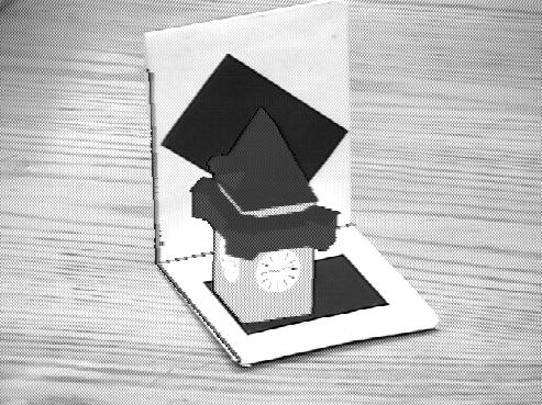
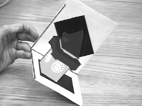
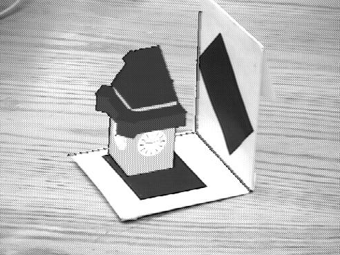
Figure 13 - Sample augmented views from U of R Augmented Reality System
2.6.3 Performance Measurements
There are two performance measures that are critical for the proper operation of an augmented reality system. First, the system must operate in real-time which we define here to be a system frequency response of at least 10 Hz. Not meeting this real-time requirement will be visibly apparent in the augmented display. Too slow update rate will cause the virtual objects to appear to jump in the scene. There will be no capability to represent smooth motion. A lag in the system response time will show as the object slipping behind the moving real scene during faster motion and then returning into place when the scene motion stops.
The second performance measure is accuracy of affine reprojection. This technique assumes that the perspective camera that is viewing the scene can be approximated by a weak perspective camera. As the camera, or affine frame, moves the changes in the projection process can be approximated by affine transformations. While this assumption is maintained the affine representation used for all components of the system will remain invariant. Any violation of the affine assumption will result in errors in the reprojection of the virtual object both in its location and shape. The affine approximation is valid under the following conditions: the distance to the object is large compared to the focal length of the lens, the difference in depth between the nearest and farthest points on the object is small compared to the focal length of the lens, and finally, the object is close to the optical axis of the lens. In addition, the affine projection matrix is computed directly from the projected locations of the affine basis points. If the trackers do not correctly report the location of the feature points in a new view of the scene then this will be reflected as errors in the affine projection matrix and result in errors in the virtual object projection.
Experiments were performed to test the performance of the system against both of these criterion. One of the concerns was the update rate attainable using sockets for communications with the tracker and graphics server. The tracker is executing on the same machine as the Matlab control script so it should be isolated from network delays. The commands going to the graphics server do go across the network however. The experiments showed that the graphics system could render the virtual image at a maximum rate of 60 Hz when running stand alone. Within the framework of the Matlab script that drives the system we were seeing a much slower update rate. Each pass through the main loop performs three operations with the graphics system: send a new affine projection matrix, request rendering of the scene and wait for acknowledgment of completion before continuing. If each of these is performed as a separate command sent to the graphics server the system executes at speeds as slow as 6 Hz depending on network activity. This is not acceptable for an augmented reality system. A modification was made to the system so that multiple commands can be sent in a single network packet. When these three commands were put into a single network transmission, the cycle time markedly improved to 60 Hz.. Needless to say, the system is now operated in a mode where as many commands as possible are transmitted in single network packets to the graphics system.
The region tracker is able to maintain better than a 30Hz update rate on the projection
matrix. It does however exhibit lags in its response. This is visible on the tracker
output by noting that the outline of the tracked regions will trail the actual image of
the region during quick motions and then catch up when the motion is slowed to a stop. An
experiment was performed to measure both the lag and accuracy of reprojection. The affine
coordinates of the white point of a nail attached to our metal frame were computed from
two views of the scene. A small virtual sphere was displayed at this location in affine
space. The augmented view was restricted to display only the output of the graphics system
yielding an image of this virtual sphere against a black background. Two correlation based
trackers were used to track the image of the nail tip in the real scene and the sphere in
the virtual image. The results of this test show a mean absolute overlay error of 1.74 and
3.47 pixels in the x and y image directions respectively over a period of 90
seconds of arbitrary rotation of the affine frame. The camera was located at the same
point where the system was initialized. Figure 14 is a plot for a section of the above
test showing results for the x axis. The plot clearly shows the delay of the
reprojection with respect to the actual point position due to lags in the system.
 Figure 14 - Plot of Actual Point
Position vs. Affine Reprojection
Figure 14 - Plot of Actual Point
Position vs. Affine Reprojection